GPS Section User's Guide

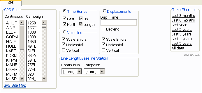
The main GPS UI looks something like this (depending somewhat on your Valve installation):

The GPS section can generate three types of plots: position time-series, velocity fields, and a displacement field. Descriptions and examples of each of these plots follow, but a word on selecting stations. Both continuous and campaign GPS stations are available to choose from (control-click/shift-click to select more than one station). Also, any single station can be set as the baseline station. This substracts that station position from all other observations. When using a baseline station only epochs in which both the source station and the baseline station have data will be used.

Position Time-Series
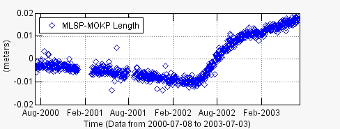
Perhaps the most common use of the GPS section is plotting time-series. Valve can plot four different components of a time-series: east, north, up, and, if a baseline station is selected, length. Here is an example of a GPS time-series:

Velocity Plots
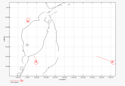
Valve can also be used to estimate velocities and plot them spatially. Select the stations you want estimated, optionally select a baseline station, choose your options, and press submit. The Scale Errors option scales the error ellipse by the model misfit, the Horizontal option draws the velocity vector, and the Vertical option shows the vertical component. Here is an example of a GPS Velocities plot at the summmit of Mauna Loa:

Displacement Plots
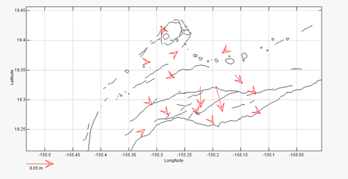
Valve can also be used to estimate a displacement at a specific time. Select the stations you want estimated, optionally select a baseline station, enter the displacement time (unfortunately this must be done by hand), choose your options, and press submit. The Detrend option removes the linear trend from the positions first, the Scale Errors option scales the error ellipse by the model misfit, the Horizontal option draws the displacement vector, and the Vertical option shows the vertical component. Here is an example of a GPS Displacement plot for a dike intrusion: